Statistics · Eqora guide
Histogram frequency density: compare the areas
Use each class width, recover counts through rectangle areas and distinguish exact class totals from within-class estimates.

Histogram frequency density matters whenever classes have different widths. A wide rectangle can contain more observations without being taller than a narrow one. If you put the raw counts on the vertical axis while also drawing the real widths, you give wide classes an extra visual advantage. The correction follows from rectangle area: divide each count by its class width so multiplying the height by the width recovers the count. Reading height alone answers a different question.
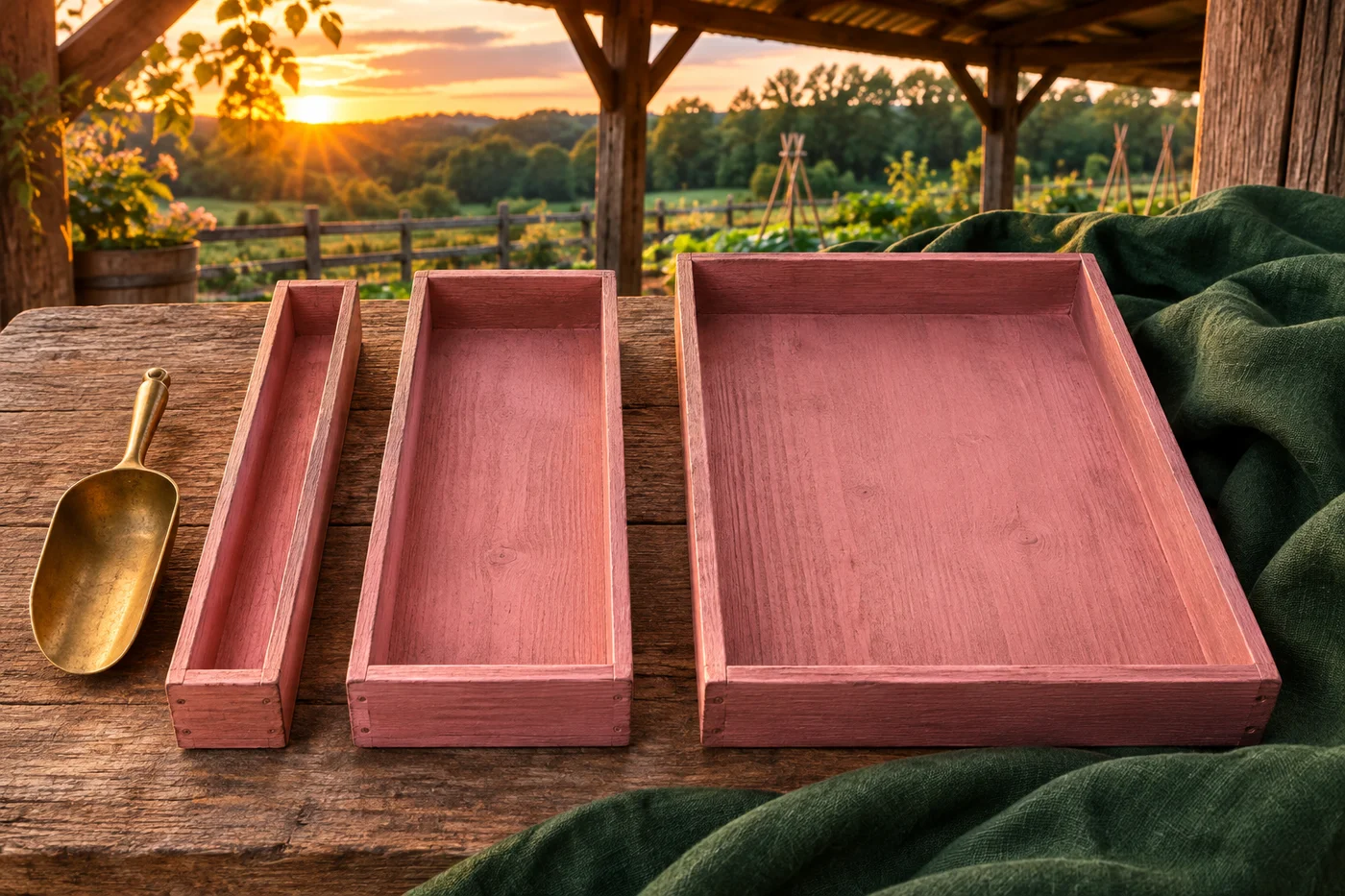
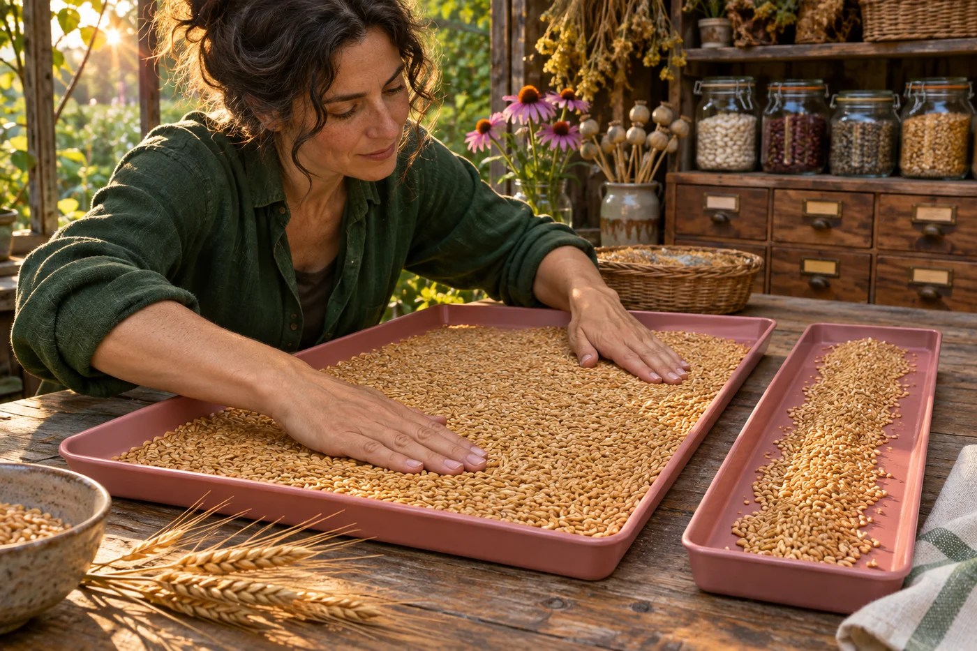
We will use a constructed sample of 100 completion times, measured in minutes, to calculate both count density and relative-frequency density. These are teaching data, not a study of Eqora users or a claim about app performance. The photographs of differently sized seed trays are conceptual analogies, not numerical histograms or evidence for the sample. You can complete the whole exercise on paper. Keep the axis labels, units, class boundaries and total count visible while deciding what each rectangle represents.
Histogram frequency density preserves the count through area
A histogram groups a numerical variable into intervals. Its horizontal positions and widths follow those intervals, so adjoining classes are drawn next to one another. Unlike a categorical bar chart, the width carries numerical meaning. When widths differ, the rectangle area must carry the frequency. With count n and class width w, choose height d = n/w. Then w × d = n. That equation explains the choice of height without relying on a special drawing convention to remember.
The Open University explanation of frequency density presents this division as frequency per unit of the variable. If time is measured in minutes, count density has units observations per minute. Multiplying by a width in minutes gives observations again. The vertical quantity is not itself the number of observations in the entire class. A height of 2 observations per minute across 20 minutes represents 40 observations. Check these units whenever a tall bar appears to conflict with a frequency table.
Set boundaries that count each observation once
Our four classes are 0 ≤ t < 10, 10 ≤ t < 20, 20 ≤ t < 40, and 40 ≤ t ≤ 60. Their counts are 20, 30, 40 and 10, respectively. The first three intervals include their left endpoint and exclude their right endpoint. The last includes 60 so the stated sample range is covered. Thus a time of exactly 20 belongs to the third class, not also to the second. Other consistent endpoint conventions are possible; read the one actually used.
The widths are upper boundary minus lower boundary: 10, 10, 20 and 20 minutes. A width does not equal the number of integers written between the endpoints. Times are numerical measurements, not a list of integer category labels. The counts sum to 100, and the intervals do not overlap. If your actual data include a value outside the stated range, the grouping needs revision rather than silent omission. Boundary checks should happen before density calculations, because a perfectly drawn histogram cannot repair an incorrectly counted table.
Calculate heights and recover every original count
Divide each count by its width. The first class has density 20/10 = 2; the second has 30/10 = 3; the third has 40/20 = 2; the fourth has 10/20 = 0.5. Draw the true interval widths along the time axis and use those four heights on an axis labelled frequency density in observations per minute. The first and third bars have the same height even though the third contains twice as many observations. Its width is also twice as large.
Now reverse the calculation: 10 × 2 = 20, 10 × 3 = 30, 20 × 2 = 40 and 20 × 0.5 = 10. The four rectangle areas sum to 100, matching the sample size. This is a stronger check than simply seeing four plausible bars. The guide to checking answers without an answer key describes why reversing a transformation helps expose a wrong multiplier. If your areas recover different counts, check whether you divided by the width, accidentally multiplied by it or used a common width for unequal intervals.
Distinguish the tallest class from the largest class total
The tallest rectangle is the second, covering 10 to under 20 minutes, with density 3. The largest class count is the third, covering 20 to under 40 minutes, with 40 observations. These statements are both correct because they compare different quantities. The tallest class has more observations per minute of interval; the wider class contains more observations in total. If a question asks which interval contains the most sample members, compare areas or table counts, not just heights.
For unequal widths, calling the tallest interval a modal class should be tied explicitly to the density convention used by the course. It does not reveal the exact most common individual completion time. Grouping has discarded the within-class arrangement. Forty observations spread across twenty minutes and thirty observations spread across ten minutes can produce the shapes we calculated, but the individual times remain unknown. State whether you mean greatest count, greatest density or an actual data mode rather than letting the word “most” hide that distinction.
Normalize the areas when the total should be one
For a relative-frequency density histogram, divide every count density by the sample size 100. The heights become 0.02, 0.03, 0.02 and 0.005 per minute. Their areas are 10 × 0.02 = 0.20, 10 × 0.03 = 0.30, 20 × 0.02 = 0.40 and 20 × 0.005 = 0.10. These sum to one. A full class area now represents the observed sample proportion, such as 0.40 or 40% in the third class, rather than the raw count 40.
A density height is not itself a probability. It carries reciprocal time units, and a normalized density can exceed one when a substantial proportion lies inside a sufficiently narrow interval. What must lie between zero and one is the area representing a probability or sample proportion over an interval. In our count-density version the total area is 100; in the normalized version it is one. Read the vertical-axis label and any scale factor before deciding whether a graph has been normalized correctly.
Know what a partial-class area assumes
The full third-class area tells us exactly that 40 of the constructed observations lie from 20 to under 40 minutes. It does not tell us how many lie from 20 to under 30. If we use the flat histogram rectangle as a uniform-within-class approximation, half the width gives an estimated count of 10 × 2 = 20. That is an estimate based on spreading the class count evenly, not an exact recovery of the original observations.
The actual count in that half could range from zero to 40 while leaving the grouped table unchanged. All forty times could fall below 30, or all could fall at or above 30 but below 40. To obtain an exact answer, use the raw observations or a finer table that records the boundary at 30. This limitation applies to reading percentiles and other within-class features too. The rectangle is a useful representation of grouped information, not proof that the underlying measured values are uniformly distributed.
Convert units without changing the represented amount
Suppose the horizontal time axis is converted from minutes to seconds. Each class width is multiplied by 60, so count-density heights must be divided by 60. The first width becomes 600 seconds and its height becomes 2/60 observations per second. Their product is still 20. Relative-frequency density changes by the same reciprocal factor. Keeping the old numerical heights while widening every interval sixtyfold would multiply the represented area by 60 and describe a different total.
A simple unit check therefore protects the whole graph. Minutes times observations per minute cancel to observations; seconds times observations per second do the same. Changing units should alter the numerical density, not the count or sample proportion. When comparing two histograms, check that they use compatible horizontal units and the same count or normalized convention. A taller bar on a graph using a different time unit is not automatically evidence of a greater concentration in the underlying data.

Keep grouping choices separate from the raw observations
Combining the first two classes gives the interval 0 to under 20 with count 50 and width 20. Its count density is 50/20 = 2.5. The area remains 50, although the previous two heights 2 and 3 have become one averaged height. That new flat rectangle hides the difference between the two original intervals. Changing bin boundaries can change the visible shape without changing a single observation, so do not treat every peak created by one grouping as a stable property of the data.
Class midpoints can support a separate approximate mean calculation: 5 × 20 + 15 × 30 + 30 × 40 + 50 × 10 = 2250, and 2250/100 = 22.5 minutes. The guide to weighted averages explains why the counts belong in those weights. Here the estimate replaces each unknown observation by its class midpoint; the actual sample mean need not equal 22.5. Grouping preserves class totals while losing individual locations, and both the graph and any midpoint summary should acknowledge that loss.
Test an altered table independently
Try classes 0 ≤ x < 5, 5 ≤ x < 15 and 15 ≤ x ≤ 30 with counts 10, 20 and 15. Their widths are 5, 10 and 15, so count-density heights are 2, 2 and 1. The first two bars have equal heights, but their areas are 10 and 20. The total area is 45. Dividing the heights by 45 gives a relative-frequency density whose areas are 10/45, 20/45 and 15/45, summing to one.
Explain why the second class contains more observations than the first without being taller. Recover each count from width times height, and name the units of the vertical axis. Eqora publishes this independent guide; an app is not required for the solution. If you consult any learning aid, verify the original table, boundary conventions, assumptions and final totals yourself. Respect assessment rules and do not treat an explanation as a guarantee of correctness or grades. A reliable interpretation states what the areas prove and what remains unknown inside each class.